Grid-free Integration

Below is the edited text and slides of a lecture Sam gave to the UCL Space Syntax Laboratory Research Seminar on 25th February 2021. Titled ‘Integration without the grid; An isovist based approach to spatial analysis’ it reflected on the work underpinning the isovist app, and discussed themes around the calculation of a key metric in the field, Integration.

[A development of this work and thinking has since been published as: McElhinney, (2024) Mean Aggregate Isovist Cascade Analysis; a temporal approach to spatial analysis. In proceedings of the 14th International Space Syntax Symposium, Nicosia]

from Eames, C., Eames, R., & Boeke, K. (1978). Powers of ten. Santa Monica, CA: Pyramid Films.

I begin with the poster from the film, ‘Powers of Ten’ by Ray and Charles Eames; in part to remind me to say thank you to Michael Benedikt, who is both a good friend and someone who invites to always ‘think better!’. He recently reminded me of the work, which stands as an invitation to think profoundly upon our existence in space, and the fluid nature of our movement in it; whether through time, scale or position. It illuminates a paradox, that whilst we experience space in a continuous, embodied and infinite nature, when we draw, measure or share it we tend to have to apply a scale, and so make it discrete and finite.

In our field, space syntax, the paradox of discretisation of space often expresses itself through ‘the graph’, of which there are two particularly common forms. These are known respectively as the axial line graph, wherein urban streets are abstracted into the longest view line of their length, and the VGA graph, in which a web of visual connectivity is approximated across the totality of an architectural space.

From both approaches it has been shown that the structures of vision captured can usefully account for navigational choices. Local measures such as connectivity, and global measures such as integration, extracted from these graphs, are known to identify properties and structures apparently relevant to the cognitive understanding of spaces. In short, they shed some light on how we learn to explore and occupy the spaces that we inhabit.

below left, axial map extracted from street map of Barnsbury, after Hillier B, Hanson J, 1984, ‘The Social Logic of Space’, Cambridge University Press, Cambridge, p124 fig 62; below right, visibility graph of a simple T space, from Turner, A; Doxa, M; O’Sullivan, D; Penn, A. (2001a). “From isovists to visibility graphs: a methodology for the analysis of architectural space”. Environment and Planning B. v28: pp.103–121; see also, E- and S-Partitions, and integration of spatial regions derived from the same, in Peponis, J; Wineman, J; Rashid, M; Hong Kim, S; Bafna, S. (1997) ‘On the description of shape and spatial configuration inside buildings: convex partitions and their local properties’;  Environment and Planning B. v24: pp. 761-781; and later more broadly in Peponis J, Bellal T. Fallingwater: The Interplay between Space and Shape. Environment and Planning B. v37: pp982-1001.

In reducing a street network to an axial line graph, we make a translational step that provides a conceptual hypothesis; that singular views and moments of change of view (turns of direction), are perceptually significant and so can be abstracted into a useful relational framework. In such a way, the axial line can safely discard pure geometry whilst retaining important perceptual information. The process of discretisation thus has a rigorous conceptual basis. Serendipitously it also produces what we might term a ‘sparse’ graph, the nodes and edges of which describe spatial configurations in a minimal form. Thus computation of ‘all to all’ metrics from the axial line graph is both efficient and efficacious. 

The decisions underlying the discretisation of a VGA graph, however, are arguably less conceptually rigorous, and to a degree can be directly linked back to the challenge (at the time) of computation of isovist geometries. Turner’s primary VGA innovation discretises the space of a plan by applying a uniform ‘grid cell’ across space as the basis for locating graph nodes. No perceptually knowledgeable step akin to the axial line application is achieved; the resulting graph of inter-visibility between all nodes is what we might term as being ‘dense’. Multiple neighbouring nodes within such graphs hold duplicated, or near identical edge connections, and computation of ‘all to all’ type global measures from them is inefficient and expensive. Such is the problem with VGA.

The Isovist, from Benedikt, M. (1979). ‘To Take Hold of Space: Isovists and Isovist Fields’. Environment and Planning B. v6: pp.47-65; above with grid cells discretised, from Psarra, S and McElhinney, S. (2014) ‘Just around the corner from where you are: Probabilistic isovist fields, inference and embodied projection’, The Journal of Space Syntax, v5: pp. 109-132

Admittedly, Turner does originally propose a ‘pragmatic’ unit of around one metre for his grid tessellation, nominating it as being one that is well related to human embodiment. Unfortunately, further methodological problems arise here. Architectural plan features often occur at scales of less than one metre, and so researchers now tend to adopt multi-various grid resolutions to suit their work. Beyond requiring exponentially extra hours of computation, such variation disregards the fact that grid resolution itself has a distortional effect on the resultant value of integration at any given point. This is challenging, to say the least, for a metric that was originally designed to allow normalised comparison between complex spatial systems.

In seeking to ‘make isovists syntactic’ Turner relegates them to the realm of being purely local units of perceptual reference, separate from topological knowledge. I happen to believe differently, that, like the axial line, they provide a primary conceptual basis for encoding and structuring a wider framework of knowledge (between both an embodied sense and an allocentric understanding), and such is the subject that I am attempting to outline.

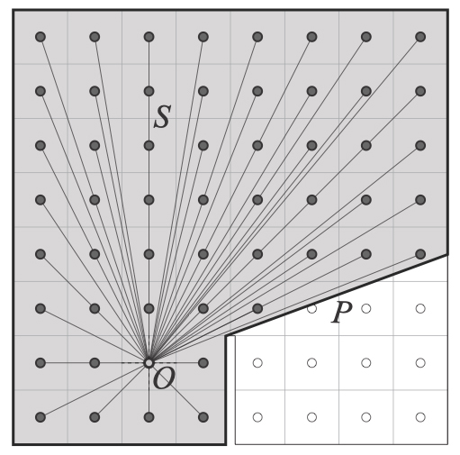
Benedikt’s original definition of the isovist as a system of points (S) visible from a vantage location (O) already implies that the isovist is not simply a geometric unit of ‘shape’ (P) but a relational one. Such an implication is entirely in line with the fact that the concept of the isovist emerged in architectural terms from the thinking of Gibson et al and the notion of the optic array.

Non intervisible isovist sub regions connected via ‘O’; from ibid

Past work that I had the pleasure of developing with Sophia Psarra at UCL built upon Benedikt’s definition, considering how a reduction of the convexity in the bounds of an isovist leads to subsets of relations within it. An isovist can then be considered as containing or bounding regions that that are internally mutually inter-visible and yet which are only related to one another via the isovist origin (S1 & S2). Such regions contain information which is either consolidated, expanded or discarded during natural movement and so they themselves encode perceptually and configurationally significant information. 

As such we have a basis for establishing relational frameworks of analysis that go beyond the purely local; instead structuring elementary relationships from regions of alternative viewpoints and co-presence within the geometrically bound configurations of multiple isovists.

Sub regions identified via sequential isovist overlap; from ibid

Such an approach does not need to be ‘grid based’. It serendipitously happens that a simple expediency of successive stochastic isovist generation, overlap and concatenation allows us to isolate such regions and develop said relational frameworks in real time. Since an isovist’s bounds are themselves pure geometric structures, the requirement for an underlying grid of discretised points for calculation is thereby entirely removed. Incidentally, watching such analysis resolve, like an analogue photo developing, can be quite instructive and enjoyable in its own right.

Below: Resolving analysis using stochastic isovists

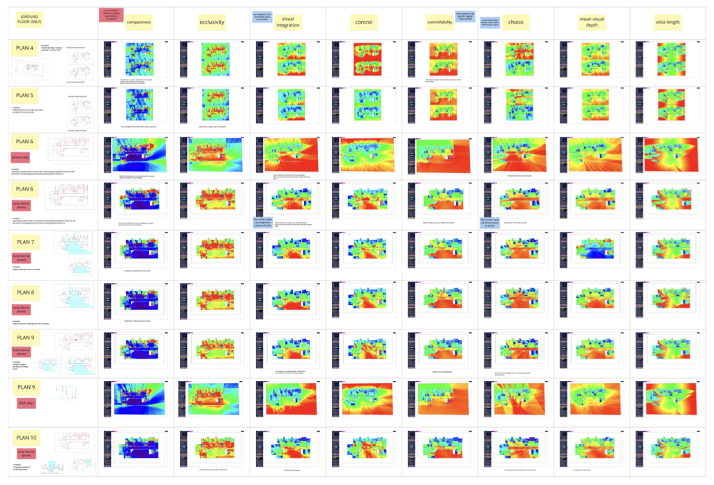
From considering such relations we now have three established measures that go beyond the purely local descriptors of isovist fields, being ‘two step’ or semi-local in measure, and bearing relation to established Space Syntax measures; directed visibility (in some instances comparable to connectivity), overt control and co-visibility. Each of these and ten other local measures (area, perimeter, compactness, occlusivity, average radial, vista length, drift, skewness, variation and curvature)  are producible in high definition in realtime in the isovist app.

Where the past work is limited is in the development of the framework of overlapping and concatenated isovist geometries to provide for fully global relations, such as integration. Again, the solution here turns out to be a simple one. Whereas for local and semi-local measures we isolate and overlap single isovists, to produce global measures we must instigate a continuous cascade of inter-linked isovists to all regions of a subject plan. Sequential stochastically rooted cascades then take the place of single isovists in the overlap and concatenation process, causing the framework of relations produced to encode global knowledge. 

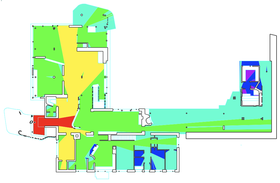
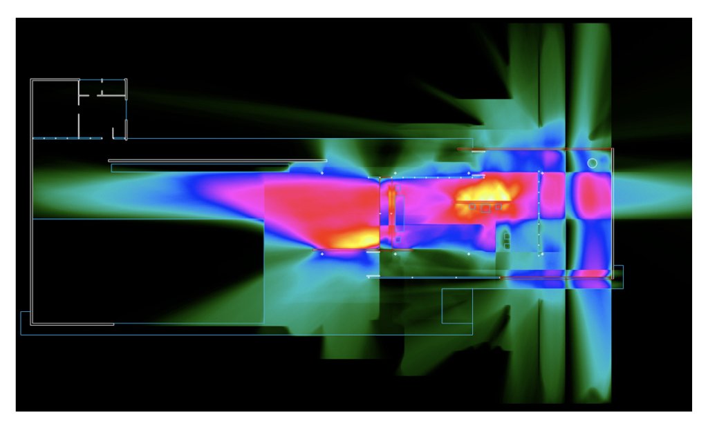
Villa Mairea, Alvar Aalto, 1939; isovist cascade from entrance to all locations in plan

Critically, it is the regions of mutual inter-visibility and potential co-presence previously identified within an isovist’s bounds that allow us to expediently construct isovist visibility cascades through a plan. Here you see one such cascade, within Aalto’s Villa Mairea. It begins at the door; the region of red on the left hand side illustrating the locations directly visible from the origin (O). From the aforementioned potential overlap regions of this single isovist we generate all possible further isovists; i.e. the next visual step, seen here as all yellow locations; and so on and so forth we continue across the totality of the plan, in this case to the deepest location, six steps from the door, in purple. Incidentally, we can record this maximum depth and average it over repeated cycles; I will return to why we might wish to do so later.

Below: Resolving Integration using isovist inter-visibility cascades

One common question, and a point which merits further examination, concerns how the metrics produced in this manner themselves become coherent. How long a ‘calculation time’ (or, how many cycles of calculation) is required to reach a stable result and does such a requirement vary, for instance, depending on plan complexity, size, or other factors?

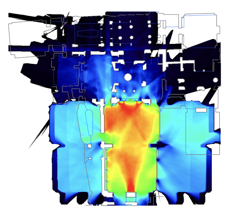
We can begin to consider said question by experimenting with the relatively simple plan of the Barcelona Pavilion. The process of resolving integration was repeated for this plan, ten times, each time allowing the resolution to develop for a total of 250 global cycles of isovist cascade and overlap. At intervals of every five cycles the value of every single data point within the plan (a total of circa 500,000 points) was recorded. At the conclusion of each 250 cycle run each of these data sets was compared to the final set of values, generating the R_Sq value (i.e. the coefficient of determination) of that data interval relative to the ultimate result. Doing so provided insights for how the data trended towards the final result over time. 

We also recorded the average value variation for all points in the plan compared to the previous cycle’s values, providing a secondary, more straightforward representation of the absolute change in results over time. 

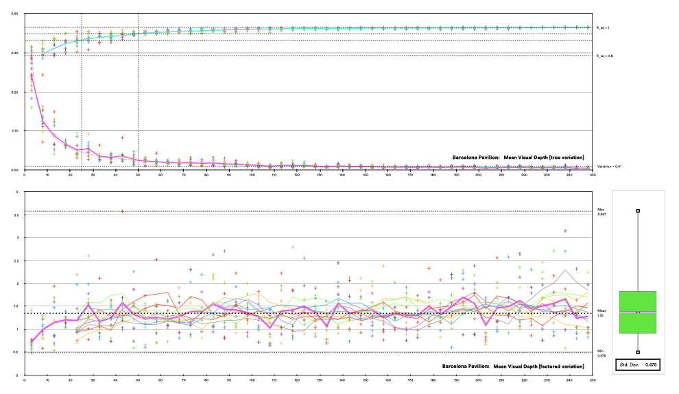
Value variations over time for integration fields in the Barcelona Pavilion

The above slide shows the results of these efforts. The r_squared value (the cyan curve) that compares the variation of the data at each cycle from the final result rapidly passes 0.8, becoming 0.9 by 25 cycles, and 0.95 by 50 cycles. In a similar way (and, in line with the averaging calculation), the average value variation (the pink curve) rapidly drops in a logarithmic curve, becoming less than 0.05 visual steps by 25 cycles.

More insightfully, we can multiply the average variation value by the number of cycles completed, to remove the effect of the ongoing ‘averaging’ calculation. Doing provides a charting of how the repeated calculation cycles themselves vary in what they contribute to the overall refinement of the integration calculation. The results of this can be seen in the lower chart, illustrating a sort of ‘jelly wobble’ of data variations around a mean figure. In the case of the Barcelona Pavilion, the mean is 1.35 visual steps, and the standard deviation that describes the ‘jelly wobble’ factor of the ongoing calculation is 0.48 visual steps.

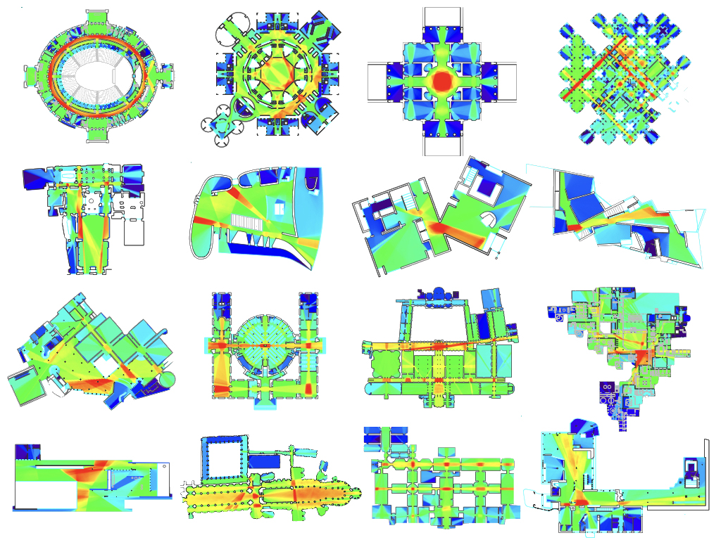
Sixteen building plan integration fields

To examine how such variation itself is influenced by different plan types, the entire process was repeated for 25 plans; ranging from basic geometries, to architectural complexes, to urban landscapes. Here are the integration fields produced; they depict high values in red, and low in blue.

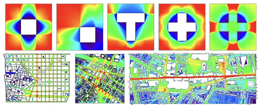
Five basic geometries and three urban landscape integration fields

The below slide shows the delta curves and the standard deviation of factored change for each plan. Estimating a typical plan data resolution of 500,000 points, overall the slide represents circa 625 million data point comparisons.

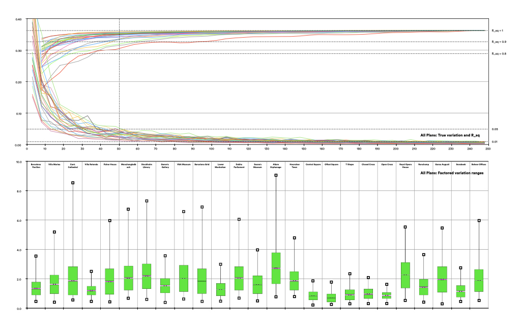
Value variations over time for integration fields in 25 different plans

One immediate and notable observation its that, for all plan types, the r_squared curve passes the 0.8 threshold by 50 calculation cycles. Mean true variation falls below 0.05 visual steps for all plan types by the same point, meaning that the numeric results are largely consistent from then on.

For the majority of plans, the former r_squared value actually surpasses 0.9 by about 25 calculation cycles; interestingly, it is the simpler geometries that lag behind the more complex ones here. Counter intuitively, complexity in a plan configuration seems to accelerate coherence in the overall calculation results; configurative influence (‘architecture’) rapidly outweighing the effect of the stochastic positioning of the origins of the isovist visibility cascades.

It is harder to discern patterns in comparing the standard deviations of the ‘jelly wobble’ factors for the variation of data in each plan type. Smaller, simpler geometries have less range of variation, which makes sense, and larger, more sprawling ones have higher variations.

Plotting the standard deviations for each plan against the average maximum depth of each plan (a factor that records the potential for variation, rather than the actual variation), allows for a further (albeit, very tentative) observation (below). Plans with looping ‘street like’ networks seem to exhibit a lower than expected deviation; whilst those with branching, room like structures return a higher than expected one. Whilst such deviation has negligible impact on the veracity of the overall integration values produced, it perhaps offers the basis for an experimental categorisation of plan typologies.

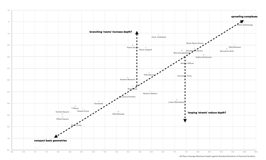
Charting Average maximum depth against standard deviation of factored variation for all plans

What, then, are the consequences of the work discussed?

Some may wish to focus on the purely pedagogic and methodological outcomes, of which there certainly are some as follows:

• Firstly, the removal of a grid graph permits a very high resolution of analysis. Being able to see in fine detail may appeal to those who wish to examine smaller elements in plan, or to begin to consider a systemic relation of things at the level of occupation and use, thus going beyond what to date has largely been a relation of spaces.
• Secondly, a more rapid route to analysis that is less finite in production invites the architectural researcher (and crucially, the designer) to adopt a more intuitive, speculative approach. Speed leads to iterative potential, and such wrapping of our techniques more directly into the design process is surely a positive broadening of our field. 
• Thirdly, we could now perhaps consider defining a standard unit of integration. If the ‘grid resolution’ that affects the K-value in the equation for integration is no more, then might alternatively tie the value for ‘K’ for any given plan to a unified measure. It probably makes sense to adopt the square metre here, as per Turner’s original suggestion.

CEPT Design Studio work using the isovist app, 2020, courtesy of Freyaan Anklesaria

Beyond these relatively technical concerns, there are wider philosophical considerations to address. To date my approach has (necessarily) limited itself to reframing established syntactic measures. Doing so has been an effort to consciously and conceptually re-align the isovist in the space syntax universe; a re-integration, if you like. The separation that has sometimes been drawn between isovists as localised units of perception, versus topological global relations of invariant spatial order can now be seen to be a false distinction that should be avoided. The relational framework that I have set out instead establishes these as a continuum, not separate branches of our field. Isovists are central to what we do, not a peripheral curiosity.

Reflections in the Barcelona Pavilion, Mies Van Der Rohe, 1929

If we accept such a positioning, then there is a consequential potential in future for the development of richer descriptors of total configurative relations of architectural space. By allowing us to take on more explicitly perceptual and embodied factors such as transparency of view, reflectivity, imagination, projection, horizon and direction, and apply them to global frameworks of relation, such approaches may in themselves offer deeper knowledge of our spaces and how we inhabit them.

Reflections in the Soane’s Museum, John Soane, 1837

Finally, we must consider the surprising alacrity by which the demonstrated methods resolve the metric of integration for all architectural plans. The rapid attainment of stability in such results from a purely stochastic sample set requires us to consider more deeply the process of exploration and the attainment of ‘sufficient knowledge’ to navigate space. It appears to be surprisingly minimal. One wonders if even fewer, strategically selected root-locations for isovist cascade may yet more rapidly cohere into navigably pertinent information. 

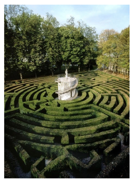
Gerolamo Frigimelica’s Maze and Folly, for Doge Alvise Pisani, Villa Pisani, Italy (circa 1720)

Ultimately, we are left with the thought that knowledge is rarely, if ever, complete and total, as discerned by the viewer in the raised central tempietto. Instead, we all exist in the maze, where our knowledge is partial and fluid, changing as surfaces flow past us, and as our views overlap with our own or those of our close acquaintances. Round and around we go; our senses of self in space and time being repeatedly made and remade in how we compile regions of embodied overlap and co-presence into individual affordances and global understandings.