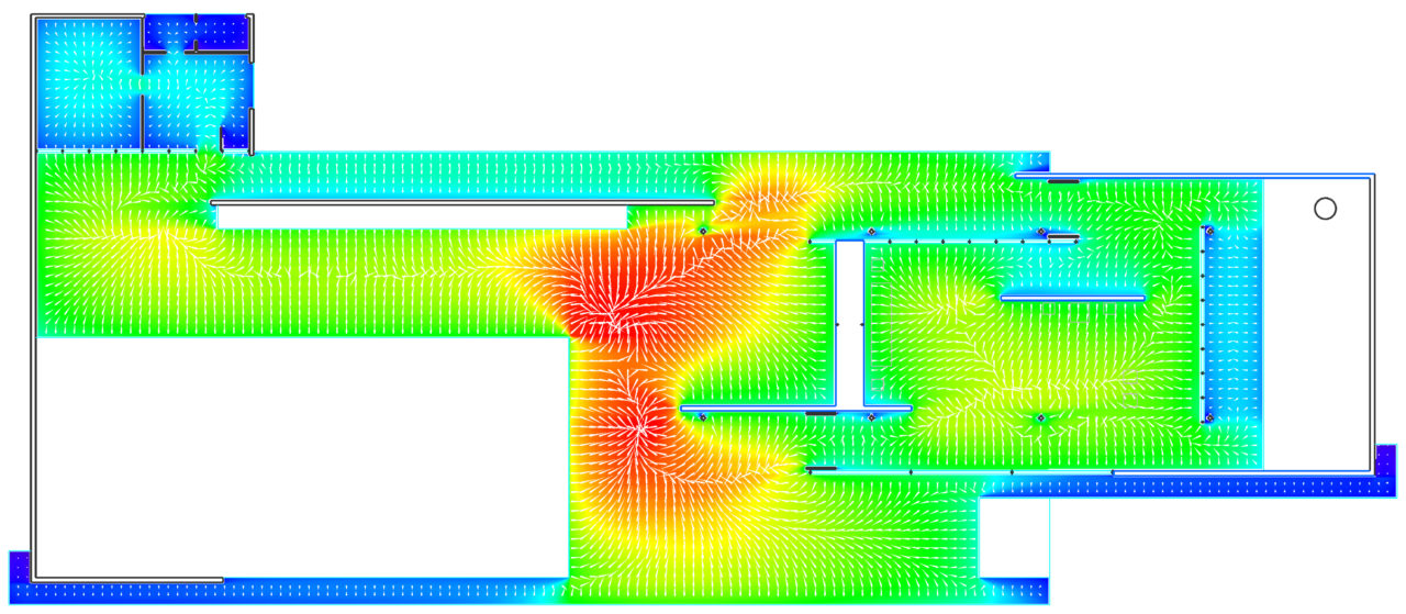
Above: Flow vectors overlaid upon an average radial field in Mies’ Barcelona Pavilion

A series of drawing overlays can be calculated and displayed over the isovist fields. To draw these:

• Import and set up a drawing for field analysis as normal.
• Open the ‘Field Analysis menu’, and run the analysis in the advanced mode if all measures are required.
• Select a field analysis for display on screen from either the ‘Isovist’ or ‘Space Syntax’ measures options. Wait… for the data representation to reach a stable condition.
• Select the ‘toggle overlays’ option and switch the required overlay type on or off:
  • Select ‘overlay absolute values’ to display point values within the field at the cursor location
  • Select ‘overlay sample locations’ to view all stochastic sample points assessed so far in the field
  • Select ‘overlay plan annotations’ to switch the drawing annotations layer on and off
  • Select ‘overlay flow vectors’ to draw a series of vector lines that indicate the direction and magnitude of the field results at locations throughout the space.
  • Select ‘overlay spatial partitions’ to display an estimated set of Peponis’ E- and S-Partitions (Peponis, 1997) based on the analysis space and isovist types.
  • Select ‘overlay persistent thresholds’ to reveal experientially key thresholds in the analysis space.
  • Select ‘overlay quad-tree grid’ to reveal the underlying search structure used to calculate visibility in the analysis space.

Below: Switching between different plan overlays in Mies’ Barcelona Pavilion